Single-shot optical surface profiling using extended depth of field 3D microscopy

Single-shot optical surface profiling using extended depth of field 3D microscopy
Pol Martinez, Carlos Bermudez,  Roger Artigas and Guillem Carles 

Abstract

The measurement of three-dimensional samples at high speed is essential for many applications, either due to the requirement for measuring samples that change fast over time, or due to the requirement of reducing the scanning time, and therefore inspection cost, in industrial environments. Conventionally, the measurement of surface topographies at high resolution typically requires an axial scanning of the sample. We report the implementation of a technique able to reconstruct surface topographies at high resolution, only from the acquisition of a single camera shot, dropping the need to perform an axial scan. A system prototype is reported and assessed as an ultra-fast optical surface profiler. We propose robust calibration and operation methods and algorithms to reconstruct surface topographies of optically-rough samples, and compare the experimental results with a reference confocal optical profiler.

1. Introduction

The precise and, specially, rapid measurement of three-dimensional surfaces is essential in many fields of science and technology. In biological research, measurement speed may be critical to capture spatio-temporal information, such as transients or dynamic events. Measurements of cell processes and dynamics of membranes may require fast particle tracking and fast topographic imaging respectively [1]. Likewise, precise surface metrology is critical in the manufacture of components in industries ranging from automative [2], additive manufacturing [3] and, above all for its significant volume, the silicon industry.

The shape, and possibly surface texture, of manufactured components usually determines their functionality and surface metrology has become an essential tool for inspection, being routinely used and adopted in these industries. Besides measurement precision, speed may be critical to push the cost per inspected part to an acceptable level.

For macroscopic imaging, techniques such as fringe projection [4] or stereoscopy provide a means of fast, single-shot data acquisition for 3D surface metrology. However, for microscopic imaging at high resolution, i.e. employing high numerical aperture (NA), the depth of field (DOF) is shallow and the main established techniques employ approaches based on optical sectioning in combination with axial scanning. In this paper, we report an ultra-fast, non-contact surface measurement technique capable of retrieving the sample topography from a single camera shot whilst using high NA optics, thus dropping the need for a time-consuming focal scan (and therefore avoiding any scanning mechanism whatsoever), and yet preserving a useful measurement range through an extension of the native DOF of the microscope.

Contact-based methods such as stylus profilers or atomic force microscopes provide the best lateral and vertical resolution and precision, however they are not exempt from disadvantages: they require repeating line scans using a tactile approach that interacts with the sample, which is not ideal, but most importantly they require a very long scanning time. Instead of this mechanical probing, optical profilers employ optical sensing to perform the measurements. Among these, imaging confocal microscopy (ICM) [5, 6], focus variation (FV) [7, 8], and coherence scanning interferometry (CSI) [9, 10] stand out as they exploit the rapid parallel measurement offered by the imaging capability of the optical head, performing areal measurements. Typically implemented into a traditional optical microscope, they are capable of providing accurate topographic measurements at the micro- and nano-meter level in a few seconds. Among these techniques, CSI provides the best vertical resolution but is very sensitive to environmental vibrations, whereas FV provides higher robustness for optically rough surfaces (as otherwise is inapplicable) but requires high numerical aperture optics to achieve satisfactory vertical resolution, and ICM provides a good balance being robust, acceptably immune to vibrations and with satisfactory vertical and lateral resolutions.

Importantly, all these techniques are based on axial scanning: the sample is scanned axially to acquire a set of optical images of the surface. In all cases, a signal that is sensitive to the presence of the surface at the focal plane is computed from the stack of images. Localising the maximum peak of this through-scan signal, called axial response, enables to identify the surface height. This is acquired and computed in parallel for all pixels, so the 3D surface of the sample under inspection can be reconstructed. Besides avoiding contact with the sample, the improved speed of optical profilers is a key advantage over contact profilers.

Nevertheless, the very requirement for sampling the axial response through a wide axial range entails three obvious implications: (a) the instrument requires a (usually expensive) means of performing the scan (a moving z-stage, tunnable optics, etc), (b) the measurement requires a full scan and therefore the associated time to complete, and (c) the measurement precision is directly affected by the precision of the stage (or of the equivalent scanning mechanism).

To improve the acquisition speed, some modifications have been proposed to avoid axial scanning in confocal microscopy. These variations include chromatic confocal microscopy (CCM), differential confocal microscopy (DCM) and dual-detection confocal microscopy (DDCM). CCM makes use of longitudinal chromatic aberration, which changes the axial focal position as a function of the wavelength, and the suppression of out-of-focus signal due to a pinhole [11, 12]. DCM places two symmetrically defocused pinholes on the detection path of the microscope [13]. The depth information is obtained from the difference in intensity detected from each pinhole, which needs to be calibrated for a particular sample reflectivity. To overcome the dependency of the sample reflectivity DDCM uses two identically focused pinholes of different sizes [14]. Depth of the sample can then be inferred from the ratio between the intensities from each pinhole.

The measurement range using CCM depends on the severity of the chromatic aberration of the objective (up to a few millimeters) and the vertical resolution depends on the wavelength discrimination capability (up to tenths of micrometers), whereas with DCM and DDCM the range of measurement is limited by the DOF of the objective. It can be extended using annular beam illumination [15], but it is effectively an apodization of the pupil aperture, but with the compromise of reducing light efficiency and limiting the vertical resolution. However, all these variations in the confocal acquisition have the disadvantage of requiring an in-plane scan (a pinhole effectively needs to be laterally scanned to reconstruct the full-field topography), limiting the acquisition time although they maintain a good confocal lateral resolution.

To perform ultra-fast topographic measurements, some techniques have been developed to reconstruct the surface topography using only a single camera shot, therefore avoiding the need for axial scanning. They typically provide measurements of lower quality (either with increased system noise, or with the appearance of measurement artifacts) but are able to provide very fast measurements. For investigations or measurements of very fast transients or dynamic phenomena, this capability may provide a means of extracting information that would otherwise be impossible. In industrial applications, they can be highly advantageous since a reduction in scanning time may drastically reduce the inspection cost to an acceptable level (in terms of cost per measured part) providing a competitive advantage.

An example of such technique is holography [16]. It is used for single-shot surface metrology, provides an ultra fast measurement, and is capable of maintaining a good lateral and vertical resolution. The disadvantage is a strict compromise between the vertical resolution and the measurement range, which is limited by the light source wavelength. The range can be extended by means of a dual wavelength light source [17] up to a few micrometers whilst maintaining sub-micrometer resolution. In addition, CCM can be modified to also work as a single-shot technology [18], although it needs to be calibrated for the spectral reflectivity of the sample.

Indeed, for single-shot techniques, the measurement range is in principle limited to the DOF of the system, and so DOF extension is a necessity for many applications. Extending the DOF can be achieved by reducing the optical aperture diameter, but this sacrifices lateral and vertical resolution besides light efficiency. Using fast tunnable lenses as a means of rapidly scanning the focal point can also effectively increase DOF, or the introduction of a controlled optical aberration in conjunction with post-detection image deconvolution [19–23]. However, extending the DOF to increase the measurement range without sacrificing vertical resolution requires an alternative mechanism by which the sample height is sensed. Engineered point spread functions (PSF) that are sensitive to the depth of the sample such as the double hellix PSF [24], tetrapod PSF [25], cropped oblique secondary astigmatism PSF [26], or parallax [27], can be used to measure height, but they require non-overlapping point-like sources or point-like illumination [28], which vastly reduces the lateral resolution (or requires lateral scanning). Extending the DOF and preserving both vertical and lateral resolutions whilst simultaneously sensing height, can be achieved by complementary kernel matching (CKM) technique [29], which implements an engineered PSF but can work at full-field, uniform illumination. The technique uses optical encoding of the imaging process such that a change in the height of the sample causes a measurable change in its image, in combination with computational recovery that exploits (and requires) the sample texture. Previously reported implementations of CKM include the use of a spatial light modulator [29] and the use of a lateral beam splitter [30] with a single camera, and combined with a complex calibration procedure. In this paper, we propose a method based on CKM that uses an implementation based on a simultaneous acquisition using two independent cameras, and employs a novel calibration and reconstruction algorithm that makes the method robust for surface metrology. We report here the experimental demonstration on a custom-made and dedicated system employing 10×/0.3NA optics that can measure surface topographies over a range of 100 µm in a single camera shot.

2. Methods

The core methodology implemented is fundamentally based on CKM [29], using a modification to work with the so-called “two-defocus” approach [30] and implemented using two independent cameras. Furthermore, a new calibration and reconstructing algorithms are reported here that result in robust measurements for surface metrology. In this section, we describe the experimental setup and the associated computational methods.

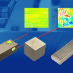
2.1. Experimental setup

The layout of the system is shown in Fig. 1. It is based on a reflected-light microscope head with two key modifications: (𝑖) the microscope objective (Nikon 20×/0.45NA) is modified to include a phase mask at its back aperture and (𝑖𝑖) a cube beam splitter is inserted between the tube lens and the image plane, that allows to install two cameras (Flir BFS-U3-51S5M-C), which are placed at different axial planes, and therefore have a relative defocus between them. The tube lens used is an achromatic doublet with 100 mm focal length. The system further includes a second beam splitter to couple the illumination, which is based on a blue LED and a condenser lens.

The phase mask has a bicubic profile and is installed at the back aperture using a plastic holder that ensures it is kept fixed in place. It also includes a fixed iris that slightly reduces the aperture of the objective to approximately 0.3NA. The phase function of the mask can be written, Φ(𝑢, 𝑣) = 2𝜋𝛼(𝑢3 + 𝑣3) (1), where (𝑢, 𝑣) are the cartesian coordinates at the pupil plane, and our phase mask has a nominal value of 𝛼 = 4.

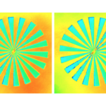
The effect of the phase mask is to modify the PSF of the system, with a number of interesting properties [31, 32]: (𝑖) the modulation-transfer function has no nulls in its spatial-frequency pass band so that image deconvolution using the measured PSF is well posed, (𝑖𝑖) the PSF is tolerant to defocus, i.e. it has a highly invariant shape over an extended DOF, (𝑖𝑖𝑖) the PSF is translated laterally as a function of defocus. This lateral shift of the PSF is produced by the employed anti-symmetric phase profile in Eq. (1) and, fundamentally, is a consequence of the known self-accelerating property of the finite-energy Airy beam upon diffraction [33], which cannot be attributed to a bending of the centre of mass but to the shape of the field [34]. Its application into incoherent imaging, as is done here, similarly yields translation of the PSF field shape through diffraction. This apparent shift of the PSF with bicubic phase modulation is proportional to square of defocus and inversely proportional to the phase mask strength 𝛼 [30, 31]. Besides defocus, the phase modulation also provides tolerance to other types of related aberrations and therefore, in conjunction with image deconvolution, it provides a mechanism to correct for aberrations [20]. An example of an experimentally recorded PSF is shown in Fig. 2(a). Overlapped and colour-coded PSFs with different amounts of defocus (taken at different axial planes) are shown in Fig. 2(b), where the shifting property is clearly evident. Using image registration with respect to the central 𝑧 = 0 µm plane, we can compute the lateral shift of the PSF at each axial plane for both cameras, which is plotted in Fig. 2(c), showing the expected parabolic behaviour. The two camera plane positions are calculated to be equally defocused.

2.2. Working principle

In CKM the depth of the sample is determined from the measurement of defocus-dependant shifts. An illustration of the operation of this windowed two-defocus CKM is presented in Fig. 3. An axial PSF stack is acquired and saved to disk, which is a one-off pre-calibration process and does not need to be repeated. For measurement, an image pair is a acquired. And for reconstruction, the acquired images are deconvolved using the series of PSFs in the stack. The result of each deconvolution is laterally shifted according to the shift of the deconvolving PSF (see Fig. 2(b)), and because the relative disparity between the PSFs of both cameras is a one-to-one function with respect to defocus (see Fig. 2(c)) the two deconvolved images will only be properly matched if the deconvolving kernel (the PSF used for deconvolution) matches the depth of the sample. Although for clarity the object in the illustration in Fig. 3 has a constant depth within the window, the reconstruction algorithm repeats the process to find the depth with best image registration at each pixel using a small neighbourhood, thus reconstructing a topography. Of course, the size of the neighbourhood is a compromise between robustness and lateral resolution.

Previous reports implementing CKM are based on a non-rigid image registration between the captured individual images. An accurate image registration is essential because in practice the sample depth is determined from measurement of defocus-dependant shifts that can be of subpixel amounts, and even modest amounts of distortion in the imaging system can affect the registration at this accuracy. To avoid this problem, we propose a different approach here. We divide the field of view in a number of windows (in this case with 11×9 windows) such that the geometrical optical distortion within one window can be assumed to be negligible. This significantly simplifies the registration problem as it can be reduced to a shift-only problem (as we outline in the next subsection), although it implies that the reconstruction needs to be computed for each window and finally stitched together.

In order to implement this approach, a custom-made array of pinholes was used so that the PSF of the system can be measured for all windows with a single image of the pinhole array. The array was fabricated using Focused Ion Beam (FIB) on a chrome-on-glass plate, where each pinhole has a diameter of 1 µm approximately and the pinhole pitch is 69 µm.

The separation between pinholes needs to be as small as possible so as to minimise within-window distortion, but big enough to avoid overlap of PSFs from adjacent pinholes. In our implementation, the size of the PSFs is of about 100 px (with some variation with defocus), and we selected a separation of 200 px as a minimum distance to accommodate the scan of PSFs including the associated lateral shifts. Because the employed camera is of 2448 px × 2048 px the field of view fits 11×9 evenly-spaced pinholes. The reconstructed field of view (ignoring marginal border areas) is therefore of 2200 px × 1800 px, corresponding to 759 µm × 621 µm at the sample. However, this is not a limitation of the technique but is set by the imaging optics (i.e. field number of the objective) and the size of the sensor. An example image of the pinhole array is shown in Fig. 4. In the next sub-sections we describe the calibration and reconstruction algorithms.

2.3. Calibration process

The calibration process simply requires the acquisition of an axial scan of the pinhole array. From these data, a calibration is computed and stored to disk, available for the reconstruction algorithm.

The measurement range is determined by the axial scan at which the calibration PSFs are acquired, but it is limited to the DOF of the system. Thanks to the effect of the cubic phase mask, the DOF of the system is extended, and therefore so is the measurement range. In our implementation we acquired PSFs through a range of 100 µm at steps of 1 µm; note that diffraction-limited DOF for 0.3NA is approximately 5 µm. We then pre-process the acquired PSFs to de-noise and store the data to disk.

The definition of the windows is not critical and can be somewhat arbitrary. In the system proposed here, the separation between pinholes is roughly 200 px and so we define a 11×9 array of windows of size 200 px × 200 px approximately centred in the field of view. The PSFs do not need to be exactly centred in each window: the deconvolution translates the image but the translation is common to images from both cameras and the relative shift is kept fixed. However, this shift is of a fixed distance with respect to each camera local coordinates, and so there are two important aspects that need to be carefully accounted for. First, the two cameras cannot be rotated with respect to each other. And second, the effective magnification for the two cameras must be the same. If these conditions are not simultaneously met, the deconvolved images will not be matching each other, even if the height of the deconvolution PSFs coincides with the object true height. The first condition could potentially be solved experimentally, adjusting the cameras with exquisite alignment, but it is in practice quite demanding because a very small rotation becomes more noticeable at field points away from the optical axis. To satisfy the second condition (same magnification for both cameras), the system needs to be perfectly image-space telecentric, because the two cameras are placed at different planes. This requires the tube lens to be placed at exactly one focal length from the exit pupil of the microscope objective, which can be done, again, with thorough experimental care. Nevertheless, instead of adjusting experimentally the system to satisfy these conditions, it is more convenient to solve the issues computationally: we calculated with high precision the relative rotation and magnification between the two cameras, and stored these parameters as part of the calibration process. This alleviates the experimental constraints, and allows for a simple and accurate shift-only registration.

To calculate the relative magnification and rotation between cameras, we used the image of the pinhole array, see Fig. 4. The entire image of the PSF array is deconvolved using a single PSF, in this case the central one. This produces an array of diffraction-limit sized spots, that can be centroided with subpixel accuracy. Repeating the process for both images we obtain a set of matching key-points between cameras. Finally, an affine transformation is found using least-squares fitting, from which we can extract the estimated rotation and magnification. Using this process we obtained a relative rotation of 𝜑 = 0.048° and a relative magnification of 𝛾 = 0.9926. These values are saved for topographic reconstruction.

The last step of the calibration is to characterise, at each window, the pinhole position as a function of the axial location at the object space. We require this information for stitching the results after reconstruction, as is explained below. To do this, we use the calculated centroids of each pinhole and adjusted a linear model to the shifts. This is justified because our implementation incorporates an iris at the back focal plane of the objective (at the same plane as the phase mask) that breaks the condition of object-space telecentricity, and so the magnification of the system has a non-negligible dependency on the axial location of the pinhole/sample. This change in magnification as we vary the axial position of the object causes a linear change in the shift in the radial direction from the optical axis. In practice, this radial distortion imparts a shift that is added to the shifts produced by the phase mask and illustrated in Fig. 2(c) (in the figure, the radial shift is suppressed because it is calculated using the pinhole at the centre of the field of view). The phase mask induced shift is isotropic (occurring in the same directions regardless of the location within the field of view) and has no significant field dependence whereas the magnification-induced shift is in the direction towards the optical axis close to the centre of the image. In any case, both contributions are directly accounted for in the reconstruction as they are included in the calibration. Nonetheless, we still require the characterisation of the magnification-induced shifts in order to assist the window stitching. We thus perform a least-squares fitting of the linear model at the shift at each window, and store the regression coefficients to disk, available for use for stitching after reconstruction.

2.4. Reconstruction algorithm

The reconstruction algorithm is based on the deconvolution of the acquired images using a series of test deconvolving kernels (based on the z-stack of PSFs acquired in the calibration step), and comparing the resultant images. The algorithm exploits the fact that the PSFs are translated differently at each camera as a function of sample height. Thus, if the height positions of both the sample and the plane used for the deconvolving kernels do not match, the two deconvolved images will be shifted with respect to each other. Conversely, if the height of the deconvolving kernels does match the sample height, the images will be properly registered. Finding the minimum of the absolute difference will therefore estimate the sample height.

The reconstruction algorithm follows the next steps for each PSF pair of the calibration process, i.e for each plane in the calibration axial scan: (𝑖) deconvolution of both acquired images,(𝑖𝑖) apply affine transformation on one image, (𝑖𝑖𝑖) subtract images, (𝑖𝑣) calculate the sum of absolute differences at a Gaussian-weighted local neighbourhood of size 𝜎 for each pixel. As mentioned above, the effect of the bicubic phase modulation prevents the appearance of nulls in the modulation transfer function which facilitates deconvolution. In our case we employed Wiener filtering using the experimental PSFs for deconvolution. Calculation of these steps for all calibration PSFs yields an axial response at each pixel, which may be used to retrieve a topography. This process is described in algorithm 1. An example of a reconstructed topography and plots of the computed axial response for selected pixel locations are shown in Fig. 5(a,b) and a topography of the sample measured with a commercial optical profiler (S neox, Sensofar) is shown in (c) for reference.

This process is however very sensitive to the lack of intensity texture at the sample, and so is prone to generate artifacts at areas without image texture. To attenuate this problem, the full reconstruction can be performed with different values of the neighbourhood size, 𝜎, yielding slightly different axial responses. In areas with sufficient texture, the result should be robust but in areas with weak signal the result is more unstable and may lead to artifacts. A high neighbourhood size enables more robust results but lower lateral resolution, and vice versa. Ideally, 𝜎 should be as small as possible but should also capture the size of the local texture features, which of course depends on the sample and may be different at different locations in the field of view. A simple solution to attenuate this effect is to independently solve the topography at a range of 𝜎 values and average the results [29].

We introduce here a more elaborated approach that aims to adapt to the size of the local image texture. The topography is reconstructed using algorithm 1 for a range of 𝜎 values (we choose a few values logarithmically spaced), and the final topography is obtained from a coarse-to-fine approach, described in algorithm 2. The algorithm starts with the largest 𝜎 to reconstruct an initial topography, and then 𝜎 is successively reduced to refine the result. The assumption is that for a large 𝜎 the reconstruction is expected to be of high quality but with lower lateral resolution, and through successive reduction of 𝜎 we increase the lateral resolution. However, if reducing 𝜎 results in a height estimation that is too different from the previous iteration, we terminate the process. The advantage of this approach is that it enables to increase resolution whilst avoiding artifacts to a higher extent, and it is locally adaptive. Examples of full topographies reconstructed using fixed values of 𝜎 compared with this coarse-to-fine algorithm are shown in Fig. 6, where it can be appreciated that if 𝜎 is too low artifacts are present and if 𝜎 is too high it smooths the topography sacrificing lateral resolution. The coarse-to-fine approach satisfactorily suppresses artifacts whilst preserving lateral resolution to a higher extent.

To reconstruct the full topography, the process is repeated at each window of the field of view, and the results are stitched together. In order to suppress stitching artifacts, the window size is defined larger than the windows pitch for reconstruction, yielding window overlap, and finally cropping the windows accordingly for stitching. Because the reconstruction follows deconvolution using the experimental image of a pinhole that may not be exactly centred at each window, a calibrated shift must be applied before stitching. Unfortunately, because this effect depends on the sample 3D shape, it cannot be incorporated into calibration, but rather requires compensation at the reconstruction stage. To solve the problem we calculate, for each window, the mean height of the reconstructed topography at the periphery of the window (i.e. the region where stitching occurs), and apply the shift that corresponds to such height, using the calibration of the shifts discussed above. Of course, if the height value along the window periphery varies significantly, this will carry errors, but we found that this solution minimises the errors whilst allowing a single shift per window.

3. Results

Reconstructed topographic measurements of a surface of a coin are shown in Fig. 7, obtained from a single camera pair shot. Note that the measurement range exceeds 100 µm, whilst the diffraction-limited DOF of the objective used at 0.3NA is approximately 5 µm. For reference, the measured areas shown in Fig. 7(a) were also measured using a commercial optical profiler (S neox, Sensofar) using the confocal technology.

Results are shown in Fig. 8 where the small artifacts from the proposed CKM implementation are visible but an overall satisfactory matching is evident. Importantly, the measurements from the confocal system followed the acquisition of a scan with 100 planes, which besides requiring the scanning mechanism (in this case a piezo scanning system) also has a much longer acquisition time compared to the single-shot operation of our implementation of CKM.

A quantitative analysis of the new approach is performed in Fig. 8 and compared to the reference confocal measurement. The feature used for the analysis is a “0” from the back face of the coin, due to its step-like nature whilst maintaining enough roughness for it to be measured with CKM. The step has been measured with the confocal technique, which resulted in a height of 34.401 µm whilst the same feature has a height of 36.320 µm with CKM. Additionally, the sample was placed at different height positions (with offsets of 10 µm, 20 µm and 30 µm) and the height values obtained were 36.425 µm, 35.804 µm and 35.780 µm, respectively.

Besides height measurements of step-like features, however, the ability to measure and characterise micro-roughness is also important in the field of surface metrology. In this aspect, the principle of measurement of the method sets limits to the lateral and vertical resolution that are possible, limiting in practice the ability to characterise micro-roughness. Height measurement is determined from the registration of intensity features, and so the lateral resolution of the topographic detail is necessarily lower than the imaging resolution. To estimate the lateral resolution, we calculated the autocorrelation length (parameter 𝑆al as defined in the ISO 25178-2) from the central flat region (after removal of the lowest spatial frequency components) in the topographies measured using our system and the commercial profiler shown in Fig. 7(c,f). For the commercial system we obtained an autocorrelation length of 𝑆al = 1.5 µm, whereas for the proposed system we obtained 𝑆al = 7.5 µm.

Since this is the same surface, the latter is an indication of the lateral resolution. As for the vertical resolution, it is also affected by the sample since the axial response (see examples in Fig. 5) has a more or less pronounced minimum depending on the sample texture, which determines the measurement precision. To provide a quantitative experimental estimation, we calculated the root mean square deviation of measurements performed on the same flat region. This measurement provides an estimation of the precision assuming that the amplitude of the surface roughness is significantly lower. Measurements using the commercial system provided a roughness parameter 𝑆q = 0.15 µm. Since this is significantly above the precision of commercial instrument, it can be attributed to the roughness of the surface. For the proposed system we obtained 𝑆q = 1.5 µm, and since it is from the same sample region, it provides an estimation of the measurement noise. Assuming that the ability to resolve small vertical changes is three times such value, it provides an estimation of the vertical resolution of 4.5 µm, which is consistent with the deviations observed for the step height measurements above.

4. Discussion 

The results shown in the previous section are overall consistent with the reference measurements performed with a commercial confocal optical profiler, although there are remaining measurement artifacts. Some of these artifacts have been filtered using a simple threshold to exclude values at each end of the height histogram. However, we have not considered a criteria to assess the quality of the axial response and classify the associated point as non-measured. This is typically done in scanning-based systems, such as the reference confocal system, using the calculated signal-to-noise ratio of the axial response. For instance, areas with high local slopes (exceeding the NA of the objective) produce axial responses of poor quality due to the reduction of captured reflected light, and lead to non-measured points. This can be appreciated in the results shown in Fig. 7 and Fig. 8. In our system, additionally, areas with insufficient texture also produce badly conditioned axial responses, i.e. without well defined minima. Implementation of an algorithm to estimate the quality of the axial response, could provide a mechanism to classify points as non-measured, potentially eliminating most of the remaining visible artifacts.

The method reported here provides single-shot acquisitions, constituting an ultra-fast technique, able to acquire the raw data necessary to reconstruct a topography in real time. However, post-detection computation is required to reconstruct a topography and its associated processing time. In our current implementation, the algorithms take 190 s to complete the processing for all 99 windows and using 10 values for 𝜎 in the coarse-to-fine algorithm. However, the method implemented here has the additional advantage of being highly parallelisable. The reconstruction of the individual topographies at each window can be computed in parallel, and because the most computationally costly operations are Fourier transforms, parallelisation can improve the reconstruction speed.

Our calibration algorithm is based on three stages: acquisition of the stack of PSFs, calibration of the affine projection from the image space of one camera to the second camera, and calibration of the pinhole shifts for window stitching. The latter two are implemented through deconvolution and centroiding of the acquired PSFs. Of course, the centroiding of point-like sources is not free from errors, and the localisation process has an associated measurement precision. Our calibration processes, however, are designed to minimise the impact of the centroiding errors through least-squares fitting: to fit the affine projection we employ the full 11×9 points to fit the affine transform which only has six degrees of freedom. Likewise, to determine the through-focus localisation of each pinhole we employ the full scan with 101 points to fit a regression line with two degrees of freedom in both horizontal and vertical image coordinates. This is a clear advantage with respect to implementations requiring non-rigid registrations, and in practice provides an improvement in accuracy of the system with respect to previous implementations.

Quantification of the accuracy is however non-trivial, as it is dependent on the sample: surfaces with highly contrasted intensity features provide a better registration signal and result in better measurement precision than surfaces with lower contrast intensity features. The method reported here is however more robust and arguably easier to calibrate and this is an improvement for profilers that need to operate outside laboratory-controlled conditions. As for the operational scanning range (i.e. the DOF achieved) our system follows the so-called two-defocus approach reported in [30] and is therefore subject to the same specifications and compromises: increasing the phase mask strength 𝛼 in Eq. (1) and a commensurate increase in defocus difference between cameras, the system DOF is increased at the expense of a lower signal-to-noise ratio in the imaging process, that ultimately affects registration accuracy and therefore measurement precision.

Because our implementation is based on the incorporation of a phase mask and iris aperture at the plane of the back aperture of the objective, the system is not object-space telecentric, as discussed above. Although this could be prevented using a different optical setup, involving a 4 𝑓 configuration to place the phase mask at a plane optically-conjugated with the aperture stop of the objective, it has the advantage of a simpler and practical implementation.

4. Conclusions

We have developed and experimentally reported a method to acquire surface topographies of rough materials, capable of reconstructing such topographies from a single camera shot with an accuracy of a few micrometers. The achieved measurement range extends to approximately 100 µm, which typically requires the acquisition of 100 images with conventional, scan-based approaches. The technique is based on the CKM method, and we have implemented a novel calibration and reconstruction algorithms that provide additional advantages. We have implemented the method in a dedicated prototype, and reported measurements of rough surfaces. The technique is based on image registration, and therefore requires image texture in a similar way that stereoscopy does. For optimal accuracy, image texture at frequencies higher than the variations in topographic detail is required. Besides some remaining artifacts and limitations in the final quality of the topographies, the single-shot capability of the technique makes it capable of reconstructing topographies with ultra-fast acquisitions, dropping the requirement to scan the sample. This can provide a solution to applications in which acquisition speed is essential, either due to movement of the sample itself (when scanning is simply not possible) or in terms of increasing the number of measured samples per second.

References

[1] H. Shen, L. J. Tauzin, R. Baiyasi, W. Wang, N. Moringo, B. Shuang, and C. F. Landes, “Single particle tracking: From theory to biophysical applications,” Chem. Rev. 117, 7331–7376 (2017).

[2] S.-C. Vlădescu, A. V. Olver, I. G. Pegg, and T. Reddyhoff, “Combined friction and wear reduction in a reciprocating contact through laser surface texturing,” Wear 358-359, 51–61 (2016).

[3] Townsend, N. Senin, L. Blunt, R. Leach, and J. Taylor, “Surface texture metrology for metal additive manufacturing: a review,” Precis. Eng. 46, 34–47 (2016).

[4] Z. Zhang, “Review of single-shot 3d shape measurement by phase calculation-based fringe projection techniques,” Opt. Lasers Eng. 50, 1097–1106 (2012).

[5] R. Artigas, Imaging Confocal Microscopy (Springer, Berlin, Heidelberg, 2011), pp. 237–286.

[6] C.-S. Kim and H. Yoo, “Three-dimensional confocal reflectance microscopy for surface metrology,” Meas. Sci.Technol. 32, 102002 (2021).

[7] S. Pertuz, D. Puig, and M. A. Garcia, “Analysis of focus measure operators for shape-from-focus,” Pattern Recognit. 46, 1415–1432 (2013).

[8] C. Bermudez, P.Martinez, C. Cadevall, and R. Artigas, “Active illumination focus variation,” in Optical Measurement Systems for Industrial Inspection XI, vol. 11056International Society for Optics and Photonics (SPIE, 2019), pp. 213 –223.

[9] S. S. C. Chim and G. S. Kino, “Phase measurements using the mirau correlation microscope,” Appl. Opt. 30, 2197–2201 (1991).

[10] A. Harasaki, J. Schmit, and J. C. Wyant, “Improved vertical-scanning interferometry,” Appl. Opt. 39, 2107–2115 (2000).

[11] S. L. Dobson, P. chen Sun, and Y. Fainman, “Diffractive lenses for chromatic confocal imaging,” Appl. Opt. 36, 4744–4748 (1997).

[12] T. Kim, S. H. Kim, D. Do, H. Yoo, and D. Gweon, “Chromatic confocal microscopy with a novel wavelength detection method using transmittance,” Opt. Express 21, 6286–6294 (2013).

[13] Y. Fainman, E. Lenz, and J. Shamir, “Optical profilometer: a new method for high sensitivity and wide dynamic range,” Appl. Opt. 21, 3200–3208 (1982).

[14] D.-R. Lee, Y.-D.Kim, D.-G.Gweon, andH.Yoo, “High speed 3d surface profilewithout axial scanning: dual-detection confocal reflectance microscopy,” Meas. Sci. Technol. 25, 125403 (2014).

[15] D.-R. Lee, D.-G. Gweon, and H. Yoo, “Annular-beam dual-detection confocal reflectance microscopy for high-speed three-dimensional surface profiling with an extended volume,” Meas. Sci. Technol. 31, 045403 (2020).

[16] M. K. Kim, “Principles and techniques of digital holographic microscopy,” SPIE Rev. 1, 1 – 51 (2010).

[17] J. Kühn, T. Colomb, F. Montfort, F. Charrière, Y. Emery, E. Cuche, P. Marquet, and C. Depeursinge, “Real-time dual-wavelength digital holographic microscopy with a single hologram acquisition,” Opt. Express 15, 7231–7242 (2007).

[18] H. J. Tiziani and H.-M. Uhde, “Three-dimensional image sensing by chromatic confocal microscopy,” Appl. Opt. 33, 1838–1843 (1994).

[19] E. R. Dowski and W. T. Cathey, “Extended depth of field through wave-front coding,” Appl. Opt. 34, 1859–1866 (1995).

[20] T. Vettenburg, N. Bustin, and A. R. Harvey, “Fidelity optimization for aberration-tolerant hybrid imaging systems,” Opt. Express 18, 9220–9228 (2010).

[21] W. Chi and N. George, “Electronic imaging using a logarithmic asphere,” Opt. Lett. 26, 875–877 (2001).

[22] S. Liu and H. Hua, “Extended depth-of-field microscopic imaging with a variable focus microscope objective,” Opt. Express 19, 353–362 (2011).

[23] P. Mouroulis, “Depth of field extension with spherical optics,” Opt. Express 16, 12995–13004 (2008).

[24] S. R. P. Pavani and R. Piestun, “High-efficiency rotating point spread functions,” Opt. Express 16, 3484–3489 (2008).

[25] Y. Shechtman, S. J. Sahl, A. S. Backer, and W. E. Moerner, “Optimal point spread function design for 3D imaging,” Phys. Rev. Lett. 113, 133902 (2014).

[26] Y. Zhou and G. Carles, “Precise 3d particle localization over large axial ranges using secondary astigmatism,” Opt. Lett. 45, 2466–2469 (2020).

[27] Y. Sun, J. D. McKenna, J. M. Murray, E. M. Ostap, and Y. E. Goldman, “Parallax: High accuracy three-dimensional single molecule tracking using split images,” Nano Lett. 9, 2676–2682 (2009).

[28] R. Gordon-Soffer, L. E. Weiss, R. Eshel, B. Ferdman, E. Nehme, M. Bercovici, and Y. Shechtman, “Microscopic scan-free surface profiling over extended axial ranges by point-spread-function engineering,” Sci. Adv. 6, eabc0332 (2020).

[29] P. Zammit, A. R. Harvey, and G. Carles, “Extended depth-of-field imaging and ranging in a snapshot,” Optica 1, 209–216 (2014).

[30] P. Zammit, A. R. Harvey, and G. Carles, “Practical single snapshot 3d imaging method with an extended depth of field,” in Imaging and Applied Optics 2015, (Optica Publishing Group, 2015), p. CT2E.2.

[31] G. Carles, “Analysis of the cubic-phase wavefront-coding function: Physical insight and selection of optimal coding strength,” Opt. Lasers Eng. 50, 1377–1382 (2012).

[32] G. Muyo and A. R. Harvey, “Decomposition of the optical transfer function: wavefront coding imaging systems,”Opt. Lett. 30, 2715–2717 (2005).