Computational self-corrected quantitative 3D topographic imaging

Computational self-corrected quantitative 3D topographic imaging
Lena Zhukova, Roger Artigas and Guillem Carles

Abstract

Three-dimensional microscopy has become an essential tool for inspecting samples across a broad range of fields, from scientific research to industrial applications. In many cases, precise geometric measurements on 3D shapes and structures at the micro scale are vital. For this, established techniques typically rely on axial scanning to sample the measured volume. However, an imperfect motion of the scanner inevitably introduces errors in the output measurements. We present a method to estimate and suppress the scanner positioning errors through computational analysis of the acquired data, leading to improved measurement precision. While methods for correction of such errors are available and well known for interferometric systems thanks to fringe analysis, this has remained an unsolved challenge for non-interferometric technologies such as confocal microscopy. We experimentally demonstrate the method and report a ten-fold improvement in the axial precision of confocal microscopy systems equipped with motorised scanners. The results are comparable to or even surpass those achieved with high-quality piezoelectric scanners, while preserving the large measurement ranges offered by motorised linear stages. Furthermore, this method offers a cost-effective alternative to high-quality scanners by leveraging low-cost computation in place of expensive hardware, and it can be seamlessly integrated into existing systems with minimal modification.

1. Introduction

Three-dimensional optical microscopy underpins our ability to observe and measure structures non-invasively at the micro and nanoscale[1,2,3,4,5]. From studying the interactions of 3D structures in life sciences[6,7,8,9] to monitoring high-precision manufacturing processes[10,11,12,13,14], imaging in three dimensions is simply essential. However, any form of imaging is a two-dimensional process, and strategies are required to accurately reconstruct three-dimensional information from acquired data. The simplest and most common approach is to scan the sample volume plane by plane, as camera-based imaging systems acquire a plane at a time, and point-scanning systems typically perform fast in-plane raster-scanning. This strategy is, in fact, felicitously convenient for high-resolution microscopy, where only a thin plane is in focus, owing to the shallow depth-of-field associated with the required high numerical aperture (NA). Ultimately, scanning is practically always required to measure three-dimensional samples.

For many fields of science, imaging is only the starting point of quantitative measurement, and 3D microscopy is no exception. For some applications, accurate localisation of 3D structures or fiducial markers can be critical. This culminates in the field of optical metrology, where high-precision measurement is its raison d’être[11]. Consequently, accurate positioning during the axial scan is paramount for any quantitative imaging, and most particularly for microscopic dimensional metrology.

Due to such high relevance, we focus our attention to high-precision 3D topographic imaging, or optical profilometry, where scanning is employed to extract spatial measurements. Indeed, optical profilometers play a crucial role in various industries such as microelectronics, biomedical engineering, and semiconductors, by providing detailed surface measurements. The operating principle is to image a region and acquire a stack of images through an axial scan. Localising the point of best focus at each image pixel yields a height map or topography of the sample. Generically, a focus-sensitive signal is sampled across the axial scan, computing the so-called axial response, and accurate localisation of its maximum peak yields the height of the imaged sample[15]. Methods to calculate such signal are the base of well-established and mature technologies, including confocal microscopy[16], focus variation[17] and interferometry[18,19].

In any scenario in which scanning is used to extend a spatial measurement dimension, errors from an imperfect motion of the scanning mechanism are directly transferred to the final 3D measurement. Therefore, reducing or correcting these errors is of utmost importance in these fields. Interestingly, this comes naturally possible in interferometry, where analysis of the phase of the fringes throughout the scan enables a high-precision monitoring of the pseudo-erratic movement of the scanner[20]. Although this is well-known in the field, it is only possible for interferometric systems, and so the problem of imperfect scanning remains unsolved for important techniques such as confocal microscopy or focus variation.

In this paper, we propose a computational method that fills this void, providing a solution to increase the accuracy and precision of scanning-based non-interferometric 3D topographic imaging systems. The method is purely computational and self-corrected in the sense that it only requires processing of the scanning data, without any need for additional hardware components. Here, we propose the concept and demonstrate an order of magnitude improvement in the precision of measurements performed with motorised linear scanners implemented in a confocal optical profiler. Such improvement has not been possible before and has only been circumvented through the use of high complexity and expensive scanners, mainly based on piezoelectric transducers. Our method enables, for example, the use of motorised linear stages with their conveniently large scanning ranges, and with a precision that matches that of piezoelectric systems.

2. Results

2.1. Problem statement

The measurement process of an optical profilometer typically includes an axial scan to localise the height of the sample at each image pixel. To perform such a scan, an ideal scanner would execute the commanded movement without errors. That is, the position of the movement coincides with the commanded (desired) position. A linear relation between the commanded and executed positions is acceptable as it would not introduce measurement errors, as long as the amplification factor can be measured and calibrated. However, a realistic scanner will introduce pseudo-random deviations from linearity that, if not accounted for, become errors directly transferred to the final 3D measurement. These are referred to as non-linearity errors of the scanner, and constitute a relevant source of imperfect precision that plagues quantitative 3D microscopy, besides other major contributors such as optical aberrations, mechanical drift, vibrations, and noise. Such deviations are behind the non-linear form of the so-called response curve of the system[21,22], a function that relates the measured position with the actual position. A response curve with exaggerated non-linearity errors is illustrated in Fig. 1a. Topographic measurements are typically obtained by computing the axial response across the scanning range to find the best focus for each pixel. Thus, non-linearity errors shift the maximum peak, leading to incorrect height values, as illustrated in Fig. 1b.

For this reason, a great deal of effort has been put into linearising the response of scanners used in high-precision systems. These include the use of piezoelectric systems with capacitive sensors for feedback control or the use of high-quality optical encoders. However, in addition to their high price, piezoelectric systems offer a limited measurement range of hundreds of micrometres, which is far from ideal for general-purpose instruments. On the other hand, motorised linear stage scanners provide large measurement ranges that suit any application, but show increased non-linearity errors. These can be attributed to a combination of inherent mechanical imperfections due to gears, actuators and guides, as well as to a varying response of the scanner to input signals due to backlash, friction, or hysteresis of the control system driving the motor. An alternative to correct non-linearity errors is to employ an independent mechanism to measure the actual scanner movement during each measurement scan, and account for them in the reconstructed measurement; however, this is often not possible.

To formulate the problem, let z=Φ(x,y) be the height map of the sample in a region in the field of view, i.e. our measurand, and ξ(z) be the response curve of the system, where (x, y, z) are the spatial coordinates in the sample volume. We can model the measurement process as,

where ϵ(x,y) is random measurement noise and the first term is the function ξ evaluated on the axial position Φ. Given that ξ is unknown, errors are embedded in the measurement, and there is no unambiguous way to separate ξ from the form of the sample surface Φ. In other words, from the measurement only, it is impossible to distinguish between the true features of the sample and the errors introduced by an imperfect scanner movement.

Of course, this would not be an issue if ξ(z) could be measured and stored as a calibration. However, the sources of non-linearity are pseudo-random and can be different on repeated measurements (see Supplementary Fig. 1). In practice this implies that a previous calibration is not possible. Fortunately, non-linearity errors associated with high-precision components are typically very small compared to the offered measurement range, and in practice it can be assumed that the corresponding response curve follows a monotonic function with modulated deviations from linearity that are smooth and of low amplitude.

The aim of the method presented here is to determine the response curve, ξ(z), from a computational analysis of the measurement scanning data. If successful, this then enables to correct for non-linearity errors, thereby greatly increasing the precision of the measurements.

2.2. Working principle of computational self-correction

The essence of the method consists in measuring a second topography of the sample, Φ′_meas (x,y), shifted by a relative vertical offset, but computed from data acquired during the same mechanical scan. This ensures the response curve ξ(z) is common for both topographies. Computing such second measurement with a vertical offset, Δz, we have,

which is also affected by non-linearity errors. These errors, nevertheless, differ from the errors affecting the first topography in Eq. (1), due to the induced vertical shift. Therefore, under the assumption that the response curve ξ(z) is unknown but deterministic, we can use these differential measurements to compute an estimation of its derivative as,

where ΔΦ_meas(z) is the difference between topographies, expressed as a function of z.

Note that if the scanning is performed without non-linearity errors, the pair of topographies would be identical except for the constant difference across the field of view. Consequently, subtracting one from the other would yield a constant value. However, if the scanning incorporates significant non-linearity errors, each computed topography will be affected by different regions of the response curve due to the vertical offset. In this case, the difference between topographies will no longer be constant but will instead become a deterministic function of the response curve, ξ(z). Moreover, since the response curve does not have a dependence on (x, y) —it is a property of the scanner—, non-linearity errors introduce a variation in the difference Φ′_meas(x, y) – Φ_meas(x, y) that depends only on the height of the sample, which we denote by ΔΦ_meas(z) in Eq.(3).

The assumption that ξ does not depend on (x, y) holds if the mechanical functioning of the scanning system is sufficiently robust to ensure rectilinear movement through scanning, which is readily achieved with standard high-precision components employed in common scanners.

The aim of the method is to use this information to estimate the response curve of the system. We achieve this by numerically determining the estimated response curve such that, when applied to correct for non-linearity errors to both topographies, i.e. inverting Eq.(1) and (2), their subtraction indeed yields the expected constant vertical offset.

In principle, numerical integration of Eq.(3) directly yields the response curve of the measurement, ξ(z). Once known, it can be used to invert Eq.(1) or Eq.(2) and solve for Φ(x,y). Since this approach attempts to correct the non-linearity errors from the topographies, using a response curve that is estimated from the uncorrected topographies, we refer to a computational self-correction.

However, the numerical calculation of the quantity ΔΦ_meas(z) from the set of noisy and (x, y)-distributed pixelated measurement points is not trivial. In order to assign every difference value to the appropriate z value, knowledge of ξ(z) would be required in the first place. In other words, a direct measurement of ΔΦ_meas from the two measurements gives ΔΦ_meas(ξ(z)) because ξ(z) is our naive observation of the height z according to Eq.(1). Thus, since ξ(z) is initially unknown, residual errors remain. Fortunately, the process can be iterated until convergence: we can calculate ΔΦ_meas, integrate Eq.(3) to obtain an estimate of ξ(z), use it to correct non-linearity errors, then calculate again ΔΦ_meas, and so on. See Methods for details.

An illustration of the process is shown in Fig.2. We use the simulated response curve (with highly exaggerated non-linearity errors for clarity) shown in Fig.1a in this example. Note that the curve is unknown beforehand and its estimation is the goal of our method. We simulate an example topography defined by Φ(x) = 0.2x, where we remove the dependency in y for clarity, without any loss of generality. Performing a noise-free measurement with a system subject to the response curve we obtain the measured topography Φ_meas(x) plotted in Fig.2a in blue. The measurement of the vertically-shifted topography Φ′_meas(x) is also plotted in (a) in orange, with Δz=10μm. It can be readily appreciated how the non-linearity errors produce differences between measurements that are higher or lower than Δz in different axial regions: for example, ΔΦ_meas is higher around the region z=38μm (i.e. x=190μm) and lower around the region z=70μm (i.e. x=350μm). This variation is shown in (b) for this illustrative example, plotted as a function of z (in blue) and also as a function of ξ(z) (in red). Note that we are interested in the former, but obtain the latter in a first iteration. If we use it to estimate ξ(z), some errors remain, but applying it to correct the measurement Φ_meas(x), we obtain an improved estimate of the true height map,Φ. As this estimate improves, so does the estimate of ξ(z). Therefore, iterating the process converges to yield ξ(z) and Φ(x).

Illustration of the self-correction method using the response curve shown in Fig. 1a. An example topography defined by Φ(x)=0.2x and measured over two different regions of the response curve separated by Δz=10μm is plotted in (a). Because they are measured through different regions of the response curve, errors are dissimilar, and the difference between measurements is not constant. (b) Calculated differences between topographies, plotted as a function of the measured height (in red) and the true height (in blue).

In the next subsections, we present a metric to experimentally quantify the severity of non-linearity errors. We then propose three different methods for acquiring the pair of topographies throughout a single scan of the motorised linear stage. Firstly, we employ a replicated detection mechanism with independent cameras adjusted with a differential focus. Secondly, we compute the two shifted topographies by differentiating the axial response of the instrument and localising the two inflection points at each side of the maximum peak. And finally, we exploit the intrinsic longitudinal chromatic aberration of the imaging system to calculate two topographies using LED illumination with different wavelengths. Importantly, the latter two approaches enable implementation of the method into existing products without hardware modification.

2.3. Assessment of performance

To experimentally assess the performance of the method, we propose to measure the 3D topographic surface of a certified step height specimen, and calculate a metric based on the measured height of the step from a series of profiles perpendicular to the step, as shown in Fig.3. Because the measurement of the step height is affected by non-linearity errors of the scanner, it will tend to be higher or lower than the true value, depending on the slope of the response curve between the two height points. Interestingly, if we tilt the specimen in the direction of the step, so that the different profiles are offset to increasing height locations, we ensure that each profile is affected by a different region of the response curve, effectively sampling the entire axial range. In this case, non-linearity errors will increase the measurement of the step height for some profiles, and reduce it for other profiles. Therefore, the severity of the non-linearity errors will increase the disparity within the measurements across profiles. Thus, as a metric of success in suppressing non-linearity errors, we calculate the standard deviation of the step height values measured for all profiles,

where and are the upper and lower measured heights of the step height in the profile i, and and are their mean across all N profiles, see Fig.3.

Assessment of the severity of non-linearity errors. A step height specimen is placed with a tilt, as illustrated in (a). The central region of the specimen is measured under highly exaggerated non-linearity errors, as shown in (b). To evaluate the errors, a series of height profiles is extracted for each row of pixels, with three example profiles drawn in (b) and plotted in (c). The plots are relative to the height of the lower side to remove the effect of the sample tilt. The plots clearly demonstrate how non-linearity errors produce different measurements of the step height difference.

2.4. Implementation using replicated detection

To experimentally demonstrate the proposed self-correction method, we built a microscope setup with a replicated image path, as depicted in Fig.4. An axial scanning system based on a motorised linear stage is used to scan the sample relative to the system. The system implements active illumination focus variation[23], employing patterned illumination projected at the sample using a transmissive mask with a chequerboard pattern through a tube lens. To obtain the axial response for each pixel, we compute a measure of the local contrast of the chequerboard pattern through the scan (see Methods for additional information). Localisation of the maximum peak of such axial response yields a height value for each pixel, rendering a topography of the sample. See Supplementary Fig.2 for a photograph of the optical setup and Supplementary Fig.3 for calibration details.

Replicated detection setup with two cameras located at different positions from the tube lens. (a) A CAD model showing the key elements of the optical setup. The sample is axially scanned, obtaining a stack of images with the chequerboard pattern projected at different axial planes. One example image of a tilted mirror as a sample is shown in (b) where the projected chequerboard pattern is visible at the in-focus region. Optical sectioning is obtained by applying the Laplacian operator, shown in (c). The complete optically sectioned stacks are shown in (d), acquired by each camera through a single scan. From these stacks, a pixel is selected, and the corresponding axial response is plotted in (e). The shift between the peaks is a consequence of the differential focus between cameras.

A beam splitter is used to replicate detection using two cameras, which are placed with a relative axial offset distance, but otherwise have identical image paths. In this way, during a single scan of the sample, the axial responses captured by each camera are approximately identical but shifted accordingly. Yet, non-linearity errors of the scanner are common. We therefore obtain a pair of topographies that meet the conditions to apply the proposed self-correction method.

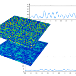
We imaged a tilted mirror, reconstructed a topography for each camera, and applied the self-correction to suppress non-linearity errors (see Methods for additional information). The difference between these topographies is shown in Fig.5a, where the ripples are indicative of non-linearity errors, while Fig.5b shows how the correction suppresses these ripples.

Differences between two topographies (a) before and (b) after correction. Previous to the self-correction, ripples affect the topography pair, resulting in a non-constant difference map. After the self-correction, the ripples are suppressed, indicating that non-linearity errors have been corrected.

To quantify the suppression, we measured a step height specimen to calculate the σSH metric defined in Eq.(4). The self-correction method provided a reduction by a factor of over 6, as shown in Fig.6, which includes a histogram plot of the step height measurement before and after computational self-correction. This indicates a great suppression of non-linearity errors, improving the measurement precision. The measured sample is a step height specimen with a certified height of 7.62μm and a certified uncertainty of 0.06μm. The results show increased precision, but self-correction does not modify or improve the accuracy of the instrument, which is generically calibrated by incorporating an amplification factor that scales the response curve. As we only focus on its linearisation, the selected relevant metric for evaluation is dispersion over measurements.

Illustration of the stochastic variability in the measurement of a step height due to non-linearity errors in the scan using the custom-built microscope. For a measurement of a tilted step height sample, the step height value is calculated for each transverse profile (see Fig.3) and the resulting measured height histogram is plotted before and after computational self-correction. Calculated dispersion values σSH are shown to quantify the reduction of non-linearity errors. The certified step height value and its certified uncertainty are (7.62±0.06) μm and are plotted with the black discontinuous line and the grey band respectively.

In this case, we deliberately induced non-linearity errors in the scan driver for increased visualisation of the correction, see Supplementary Note 3 and Supplementary Fig.4 for details. In the next subsection, we demonstrate the method on a compact, table-top system.

2.5. Implementation on state-of-the-art instruments

For a more practical application, we also implemented the method on a commercial confocal optical profiler (S neox, Sensofar) equipped with a motorised linear stage. Experiments were conducted using a 20X/0.45 NA microscope objective. In this case, replicated detection using two cameras is not an option, thus we propose two alternative mechanisms to acquire the pair of topographies required for the self-correction, from a single scan and using a single camera. The used measurement parameters correspond to the default configuration of the system.

Differentiation of the axial response

Generally, the height at each pixel of a measurement using an optical profilometer is typically found by fitting a curve to a few sampling points around the location of the maximum value of the axial response. Here, we instead propose to localise the two points of inflection of the axial response around its peak. This provides a means for computing two axially-shifted topographies from a single scan[24], that may be used as input in the proposed method. To do this, we differentiate the axial response and localise the resulting peaks (see Methods). An experimental example is shown in Fig.7 for illustration, and more details are provided in Supplementary Note 4 and Supplementary Fig. 5.

However, the width of the axial response, and therefore the axial shift between these topographies, may not be constant across the field of view, even in the absence of non-linearity errors. This violates the critical assumption that ξ(z) does not have a dependence on (x, y). Indeed, even mild optical aberrations that are field-dependent cause a variation in the difference between the pair of topographies. This can be appreciated in the experimental example shown in Fig.7. Besides optical aberrations, other effects induced by the sample can cause a variation in the width of the axial response. For example, reflective samples with significant local slopes effectively cause a reduction of the system NA (as light reflected off a large angle is not captured through the objective pupil), altering the width of the axial response. In all, this implies that the vertical offset in Eq.(2) cannot be assumed to be constant, but has a particular field dependence. To solve this, we need to measure or estimate such axial shift Δz(x,y) across the field of view, and incorporate it into the reconstruction algorithm. See Methods for a description and more details of the estimation of Δz(x,y) from the measurement data.

We measured the step height specimen to assess the self-correction, and achieved an order of magnitude reduction in the σSH metric. This indicates a great suppression of scanner errors, as shown in Fig.9.

Map of differences between two topographies obtained through differentiation of the axial response. The axial responses and corresponding derivatives are plotted for two selected pixels. The width of the axial response, and therefore the separation between peaks of the derivative, changes for different locations in the field of view.

Using multiple illumination

We propose to obtain multiple topographies by using LED illumination with different central wavelengths[25]. Due to a small but measurable longitudinal chromatic aberration, the focal point exhibits a slight displacement for different wavelengths. This can be exploited to acquire two axially-shifted topographies through a single scan. At each scanning step, simple electronic control is used to rapidly illuminate the sample with alternating LEDs, thereby acquiring the data necessary for the reconstruction of multiple topographies through a single scan.

As in the previous approach, Δz(x,y) has a field dependence that we need to estimate and incorporate into the self-correction algorithm. In particular, Δz(x,y) corresponds to the difference in flatness deviation caused by field curvature of the system for the two illumination LEDs. We chose to use blue and green LEDs for illumination, available in the optical profiler, with central wavelengths of λ=520nm and λ=455nm respectively. A measurement of a flat mirror that highlights the difference in field curvature and the resulting Δz(x,y) is shown in Fig.8. Besides the variation in focal plane and field curvature, there might be a difference in magnification that, if significant, might add errors in the calculation of the difference between topographies. However, typical dimensional scales in microscopic topographic imaging are many times larger in the lateral dimension than in the axial dimension, and so for well corrected objectives this is not significant. In particular, for the objective employed here, we observed a lateral distortion below 0.2% across the entire field of view, which has minimal impact, and becomes practically nonexistent towards the centre of the field of view.

(a) Flatness deviation caused by optical field curvature for green and blue LEDs, and (b) their difference across the field of view yielding Δz(x,y).

The results of repeated measurement of the step height, for all profiles as described in Fig.3, are shown in the histogram plot in Fig.9. The suppression of non-linearity errors decreases the dispersion across measurements, which is quantified through the metric σSH, shown for each case. Results for the commercial optical profiler are shown in Fig.9 for the cases of: uncorrected data using the linear stage scanner (in red), self-corrected using differentiation of the axial response (in blue), self-corrected using multiple illumination (in yellow), and results acquired using the high-quality piezoelectric scanner available in the commercial instrument for reference (in green). In both cases, self-correction provides a great reduction of non-linearity errors, yielding a reduced σSH metric. Equally to the results presented in the previous Section, self-correction suppresses non-linearity errors, and we focus on precision rather than accuracy to assess linearisation of the response curve.

Illustration of the stochastic variability in the measurement of a step height due to non-linearity errors in the scan using the commercial profilometer. For a measurement of a tilted step height sample, the step height value is calculated for each transverse profile (see Fig.3) and the resulting measured height histogram is plotted for different cases: uncorrected, corrected using axial response differentiation (ARD), corrected using multiple illumination (MI), and using the piezoelectric scanner for reference. Calculated dispersion values σSH are shown to quantify the reduction of non-linearity errors. The certified step height value and its certified uncertainty are (7.62±0.06) μm and are plotted with the black discontinuous line and the grey band respectively.

So far, we have applied self-correction to step height specimens, because they allow for easy quantification of the improvement. In practice, it is desirable to apply the correction to samples with an arbitrary surface form. For example, the local slope of the surface at each location within the field of view, can affect the shape of the axial response and, therefore, the operation of self-correction. An interesting example, to further evaluate the performance of the algorithm, is the measurement of spheres. The large measurement range required to measure spheres makes the presence of non-linearity errors practically inevitable. Example results of a sphere measurement are presented in Fig.10. In this case, multiple illumination was used to perform computational self-correction. The reconstructed topography is rendered in (a), with the shown profile plotted in (b) for the cases of green and blue illumination, and the difference is plotted in (c). As can be observed, the differences are not constant. In this case, the variations arise not only from non-linearity errors but also from field variations due to aberrations. After estimation of the field-correction term and application of self-correction, the differences appear flattened, shown in (d) and (e) respectively. Additionally, we removed a best-fit sphere from each topographic reconstruction, and the results are plotted in (f). The results are not perfectly flat, as expected, due to the so-called residual flatness errors associated with the sample shape[26,27]. However, we also include in (f) the results of the measurement using the piezoelectric scanner, and the results show great agreement. Despite non-linearity errors are generally corrected, there is a remaining lower-order error that vanishes at the centre but is noticeable at the edges, which we attribute to an imperfect estimation of the field-correction term. In all, this demonstrates the effectiveness of the method to correct for non-linearity errors.

Self-correction method applied on a sphere using multiple illumination with blue and green LEDs. (a) Surface topography of the measured region of a sphere. A cross-section profile is extracted from the topography and shown in (b) for both topographies using blue and green LED illumination. The differences between these profiles are plotted in (c), revealing non-flat variations. A field-correction term is estimated to reduce the field dependency, and is shown in (d). After applying the field-correction term, the differences between the topographies are flattened, as seen in (e). Finally, a best-fit sphere is subtracted from each measurement, and the corresponding residuals are shown in (f). The similarity between the self-corrected results and the results obtained with the piezoelectric scanner indicates satisfactory suppression of non-linearity errors.

3. Methods

3.1. Topography reconstruction

For the implementation using replicated detection on the custom-built microscope, we implemented focus variation with active illumination. For this, a chequerboard illumination pattern is projected onto the sample through the microscope objective (Nikon 20/0.45NA). We scan the sample using a motorised stage (PI miCos, LS-120) and acquire an image at each scanning step. To calculate the axial response (a) we apply a Laplacian filtering to the acquired image, and then (b) we apply a Gaussian smoothing filter with σ=3 pixels. Repeating these operations at each axial plane (i.e each acquired image) provides the axial response for each pixel. The Laplacian operator detects high spatial-frequency components, and in particular the sharp edges of the projected chequerboard pattern, effectively responding to focus, while the Gaussian smoothing is applied after to remove the texture of the projected pattern. The value of σ is chosen to match the size of the chequerboard, which should be small enough to not excessively sacrifice lateral resolution. An example is included in Fig.4b,c showing how the output effectively detects focus: higher signal in (c) is obtained at in-focus regions where the chequerboard pattern is visible in the raw image (b). The resulting signal therefore renders the axial response for each pixel, which is sensitive to focus. For localisation of the maximum peak, we fit a Gaussian curve to the 3 data points around the maximum peak. For the reported experiments, we scan a total range of 60μm at a step size of 1μm.

For the experiments performed with the commercial system (S neox, Sensofar) the confocal mode of the system was used, consisting of the projection of structured light to obtain optical sectioning[28]. A full range scan of 60μm was performed at a step size of 0.4μm. The system is equipped with a motorised stage and a piezoelectric scanner, allowing to acquire measurements using both technologies for comparison. The experiments were performed using a 20/0.45NA microscope objective, and the motorised stage, to enable large scanning range and demonstrate non-linearity error correction.

For the implementation relying on the smoothing and differentiation of the axial response, we applied Savitzky–Golay[29] filters, which perform a polynomial fit to a window of data points. The smoothing filter fits a polynomial of order 3 to a sliding window of 2m₂ + 1 points, where m₂, is the half-window size. In this study, we used m₂ = 7, corresponding to a total window size of 15 points. For computing the derivative, the Savitzky–Golay filter calculates the slope of the fitted polynomial at the central point of each window. To compute the numerical derivative m₂ = 7 was also used. See Supplementary Note 4 and Supplementary Fig.5 for further details and illustration.

Finally, we apply a Gaussian smoothing (σ=3) to the reconstructed topographies to reduce noise.

3.2. Iterative self-correction

We initially calculate the difference between the two measured topographies,

where we explicitly indicate a sole dependency in z, and F(x, y) accounts for a variation of Δz in different (x, y) locations. If Δz in Eq.(2) is constant for all (x, y), then the difference only depends on ξ(z), it is independent of (x, y), and F(x, y) vanishes. If, on the other hand, Δz has a dependency in (x, y), then the residual term F(x, y) is defined such that it captures the dependency in (x, y) and has a null average across the field of view. We discuss how to estimate F(x, y) in the next subsection.

To calculate the difference between topographies from our two pixelated topographic measurements, we divide the measurement axial range into equally distributed bins, centred at locations z_i , and we calculate the average value of Eq.(5) for all pixels that fall in each bin. That is,

where the summation at each bin i is taken over all pixels that satisfy,

where Φ(x,y) is the corrected topography, 2δz=z_i −z_i−1 is the width of the bins, and N_i is the number of pixels in the bin i. Note that the sampled differences are binned according to the corrected topography Φ(x,y), which is initially unknown, but it can be estimated if we have an estimate of ξ(z), by inversion of Eq.(1).

We pose the problem as an iterative process. At iteration n we calculate the corrected topographies using the current estimate of the response curve ξ_n(z) as,

initiating the response curve as the identity function, i.e. ξ₀ (z)=z.

We use Φ_n(x,y) in the condition (7) to update our estimate of ΔΦ_meas(z) using Eq.(6), which we denote by ΔΦ_n(z). The response curve for the next iteration can be obtained by integrating,

Equations (8) and (9) provide Φ(x,y) given ξ(z), and Equations (6), (7), and (10) provide ξ(z) given Φ(x,y), and so these can be iterated until convergence. Note that on ξ_n(z) converging to the true response curve ξ(z), the differences ΔΦ_n(z) converge to Δz for all (x, y). In other words, the difference between corrected topographies flattens. In this condition, non-linearity errors have been successfully corrected.

In the next subsections we describe the numerical integration, and the binning process. For an overview of the complete algorithm, refer to Algorithm 1 included in the Supplementary Information.

3.3. Estimation of the response curve from differential measurements

To calculate ξ(z) from a given set of values ΔΦ_i we perform a numerical integration of Eq.(10). However, because Δz cannot be in practice arbitrarily small, some numerical care is required. We perform the integration by building up the sampled response curve ξ(z_i ) at increasing values z_i. These are the same locations used to sample ΔΦ_i in Eq.(6). Starting with the lowest location z₀, and following a bottom-up approach, we calculate successive samples of the response curve as,

where the value ξ_ini (z_i – Δz) is linearly interpolated using ξ_ini (z_j) and ξ_ini (z_j+1), where z_j is the highest value that satisfies z_j < z_i – Δz. This bottom-up approach is illustrated in Fig.11.

Illustration of the numerical integration to obtain the response curve from differential measurements. The response curve is initiated at ξ(z₀ )= ΔΦ₀ and at successively higher z₁ locations we calculate ξ(z_i ) from ΔΦ_i . In the drawing, the sample at z₁ is being calculated, and the result is plotted with the blue dot, and black dots represent samples solved in previous steps. For the initial region for which ξ(z_i – Δz) is not available, the value is linearly extrapolated and illustrated by the dotted orange line.

However, the linear extrapolation used in the initial points z_i < z₀ + Δz might add a deviation from the actual response curve that is carried to subsequent calculations. Fortunately, this deviation gets increasingly attenuated as we proceed in calculating ξ(z_i) for increasing z_i. To solve this, we repeat the operation starting from the highest z_i and calculate ξ(z_i) for successively decreasing z_i samples as,

where z_last is the highest z_i, and ξ_ini is only used at the highest z region where the deviation is maximally suppressed.

3.4. Estimation of the field variation of the axial distance

As mentioned, the implementation of our self-correction algorithm might need to be applied using input topographies that have an axial shift that varies across the field of view, Δz (x,y). It is imperative to account for this dependence in Eq.(3) before attempting numerical integration to retrieve the response curve ξ(z). Unfortunately, because the properties of the sample itself affect the form of such field variation, it cannot be calibrated beforehand.

To account for Δz (x,y) we add the field-correction term F(x, y) in Eq.(5). To calculate F(x, y), we compute ΔΦ_meas (z) using the binning process described by Eq.(6) and, additionally, we define a disparity measure that calculates the standard deviation of the values within each bin as,

Interestingly, if F(x,y) does not adequately capture the dependency in (x, y), the values assigned to each bin would be more dissimilar, increasing the values S_i. Therefore, a good estimate of F(x, y) should minimise S_i, as shown on Supplementary Fig. 7. On the other hand, we expect F(x, y) to have a smooth variation. To satisfy this and prevent overfitting, we define F(x, y) as,

where Zⁿ_m are Zernike polynomials.
​
We find the coefficients α^m_n by minimisation of Eq.(13), effectively decoupling the dependence in (x, y) from z (see Supplementary Note 7 for more details). That is,

Calculation of values S_i and therefore the resulting values α^m_n in principle depend on the binning condition (7), and so the process should be included in the main iterative procedure. However, in practice, calculation of F(x, y) is robust and suffices to use the estimate in the first iteration. This saves computational burden, as minimisation in Eq.(15) is computationally expensive.

In our experimental implementations, we found that using Zernike polynomials up to order n=2 provides satisfactory results. This means that (ignoring the piston term α⁰₀) the field dependence F(x, y) is fully described by 5 parameters α^m_n . For additional information, see Supplementary Figures 7 and 8 for a visual representation of the estimation of the field-correction term and the selected Zernike polynomials.

4. Discussion

We have developed a self-correction algorithm capable of greatly reducing non-linearity errors in the scanning mechanism of 3D microscopy. The approach is computationally self-corrected in the sense that such errors are calculated using the same data that are used for the 3D reconstruction. The technique can be implemented in existing devices without hardware modifications and without any compromise.

Of course, the technique can only self-correct for non-linearity errors in the regions where there are data to correct for. That is, it can only correct for the axial regions that are occupied by the sample for some locations in the field of view. In principle, this is not a limitation in the sense that errors outside the measurement range occupied by the sample are in fact irrelevant. However, if the sample has gaps in its continuum of height values, errors in these gap regions cannot be calculated, and the relative height between height-disconnected regions is still affected by remaining non-linearity errors in the gap region. In other words, the technique requires the histogram of heights of the sample to be continuously filled throughout the range of interest. If this is not fulfilled, such that the histogram of the heights of the sample contains gaps, then non-linearity errors cannot be estimated in these gap regions. This is the case for example on measuring step height samples, which have a histogram consisting of two peaks. This problem however can be solved by tilting the sample, as we have done in our experiments. If this is not possible, the method can still be applied, however the response curve for those regions would be interpolated to fill in the gaps.

The goal of the proposed method is to linearise the response curve of the instrument, and we have demonstrated a great reduction of non-linearity errors. However, the method cannot measure and correct for the amplification factor, i.e. the slope of the response curve. The amplification factor is typically calibrated by measurement of a certified specimen, and our method assumes that the response curve deviates locally from the linear form but otherwise has an amplification factor that can be calibrated. This is tightly related to the choice of the axial shift Δz used in the reconstruction. Larger or smaller values than the actual implemented shift, would directly modify the resultant amplification factor of the estimated response curve. Since the aim of the method is the linearisation of the response curve, the discussion of the presented results is on precision, rather than accuracy, assessed here as the dispersion over repeated measurements.

The axial shift Δz is used to perform the differential measurement and estimate the derivative of the axial response. Because this distance is not infinitesimally small, it limits the calculation to slow variations in the slope, which is convenient because the higher-amplitude modulations of the non-linearity errors are typically of lower frequency.

We have demonstrated the method using three approaches for obtaining the required topography pair: (a) using replicated detection, (b) by differentiating the axial response, and (c) using multiple illumination. The first method provides the advantage that the axial shift between the pair of topographies is fixed (it does not depend on the sample shape, material, tilt, etc.) however it requires a modified hardware with two cameras and a beam splitter. Although a calibration step to build a map between the local coordinates of the two cameras is required, this is not complicated and this approach results in a robust implementation. The second implementation, based on differentiation of the axial response, has the advantage of not requiring any modification at all, it can be applied directly to improve topographic measurements from the dataset that is conventionally acquired. However, we have observed that to achieve robust results, a denser axial sampling is recommended as otherwise we observed periodic artifacts in the reconstructed topographies (see Supplementary Note 5). For this reason we decided to sample the axial response at steps of 0.4μm with the 20X/0.45NA objective, which results in a higher number of acquired images (the commercial system used for the experiments implements a step size of 1μm for this objective). Finally, the multiple illumination approach has the obvious requirement of acquiring two images at each step. Additionally, the convenience that a small longitudinal chromatic aberration results in a useful axial shift for two different colour bands is in principle not guaranteed, as it depends on the actual optical performance of the microscope objective, although it is highly likely, as is demonstrated here. In all, the multiple illumination approach appears to be more robust for different conditions and for calculating the field-correction term. For example, if the shape of the axial response is affected by the sample (for example by its shape, material or tilt), the localisation of the peaks for two wavelengths can be more robust than a measurement based on calculating the width of a single axial response.

5. Data availability

The datasets used and/or analysed in the current study are available from the corresponding author upon reasonable request.

6. References

[1] Stephens, D. J. & Allan, V. J. Light microscopy techniques for live cell imaging. Science 300, 82–86 (2003).

[2] Zhang, J. et al. Optical sectioning methods in three-dimensional bioimaging. Light: Sci. Appl. 14, 11 (2025).

[3] Conchello, J.-A. & Lichtman, J. W. Optical sectioning microscopy. Nat. Methods 2, 920–931 (2005).

[4] Huisken, J. & Stainier, D. Y. R. Selective plane illumination microscopy techniques in developmental biology. Development 136, 1963–1975 (2009).

[5] Leach, R. K. Optical Measurement of Surface Topography (Springer, 2011).

[6] Chen, B.-C. et al. Lattice light-sheet microscopy: Imaging molecules to embryos at high spatiotemporal resolution. Science 346, 1257998 (2014).

[7] Göbel, W., Kampa, B. M. & Helmchen, F. Imaging cellular network dynamics in three dimensions using fast 3D laser scanning. Nat. Methods 4, 73–79 (2007).

[8] Huisken, J., Swoger, J., Bene, F. D., Wittbrodt, J. & Stelzer, E. H. K. Optical sectioning deep inside live embryos by selective plane illumination microscopy. Science 305, 1007–1009 (2004).

[9] Grewe, B. F., Langer, D., Kasper, H., Kampa, B. M. & Helmchen, F. High-speed in vivo calcium imaging reveals neuronal network activity with near-millisecond precision. Nat. Methods 7, 399–405 (2010).

[10] Gao, W. et al. On-machine and in-process surface metrology for precision manufacturing. CIRP Ann. 68, 843–866 (2019).

[11] Leach, R. Characterisation of Areal Surface Texture (Springer, 2013).

[12] Zuo, C. et al. Deep learning in optical metrology: A review. Light: Sci. Appl. 11, 39 (2010).

[13] de Groot, P. J., Deck, L. L., Su, R. & Osten, W. Contributions of holography to the advancement of interferometric measurements of surface topography. Light: Adv. Manuf. 3, 258 (2022).

[14] Li, D., Wang, B., Tong, Z., Blunt, L. & Jiang, X. On-machine surface measurement and applications for ultra-precision machining: A state-of-the-art review. Int. J. Adv. Manuf. Technol. 104, 831–847 (2019).

[15] Leach, R. Advances in Optical Surface Texture Metrology (IOP Publishing, 2020).

[16] Artigas, R. Imaging confocal microscopy. In Advances in Optical Surface Texture Metrology, 2053–2563, 4–1 to 4–33 (IOP Publishing, 2020).

[17] Repitsch, C., Zangl, K., Helmli, F. & Danzl, R. Focus variation. In Advances in Optical Surface Texture Metrology, 2053–2563, 3–1 to 3–30 (IOP Publishing, 2020).

[18] Su, R. Coherence scanning interferometry. In Advances in Optical Surface Texture Metrology, 2053–2563, 2–1 to 2–27 (IOP Publishing, 2020).

[19] de Groot, P. Coherence Scanning Interferometry 187–208 (Springer, 2011).

[20] Schmit, J. & Olszak, A. G. Challenges in white-light phase-shifting interferometry. In Interferometry XI: Techniques and Analysis (Vol 4777, 118–127). International Society for Optics and Photonics (SPIE, 2002).

[21] International Organization for Standardization. ISO 25178–600:2019 – Geometrical product specifications (GPS) – Surface texture: Areal—Part 600: Metrological characteristics for areal topography measuring methods (Tech. Rep, ISO, 2019).

[22] Leach, R., Haitjema, H., Su, R. & Thompson, A. Metrological characteristics for the calibration of surface topography measuring instruments: A review. Meas. Sci. Technol. 32, 032001 (2020).

[23] Bermudez, C., Martinez, P., Cadevall, C. & Artigas, R. Active illumination focus variation. In Optical Measurement Systems for Industrial Inspection XI, Vol. 11056, 110560W. International Society for Optics and Photonics (SPIE, 2019).

[24] Zhukova, L., Artigas, R. & Carles, G. Computational self-correction of scanning nonlinearities in optical profilometry. In Optical Measurement Systems for Industrial Inspection XIII, Vol. 12618, 126180V. International Society for Optics and Photonics (SPIE, 2023).

[25] Zhukova, L., Artigas, R. & Carles, G. Suppression of scanning nonlinearities through computational self-correction in optical profilometry. In Optics and Photonics for Advanced Dimensional Metrology III, Vol. 12997, 129970H. International Society for Optics and Photonics (SPIE, 2024).

[26] Bermudez, C. et al. Residual flatness error correction in three-dimensional imaging confocal microscopes. In Optical Micro- and Nanometrology VII, Vol. 10678, 106780M. International Society for Optics and Photonics (SPIE, 2018).

[27] Giusca, C. L., Leach, R. K., Helary, F., Gutauskas, T. & Nimishakavi, L. Calibration of the scales of areal surface topography-measuring instruments: Part 1. Measurement noise and residual flatness. Meas. Sci. Technol. 23, 035008 (2012).

[28] Neil, M. A. A., Juškaitis, R. & Wilson, T. Method of obtaining optical sectioning by using structured light in a conventional microscope. Opt. Lett. 22, 1905–1907 (1997).

[29] Savitzky, A. & Golay, M. J. E. Smoothing and differentiation of data by simplified least squares procedures. Analyt. Chem. 36, 1627–1639 (1964).